A Git repository was created to host some data files, in various formats. As a first step, you will have to make a local copy of this repository on your computer, and turn it into an Rstudio project.
Download the whole content of the repo as a zip file, and unzip it in a given folder on your computer.
Open Rstudio, and open the menu File > New Project.
Choose the type “Existing directory”, and create a project in the folder created in step 1.
2.2 Usual data formats in morphometrics
Usually, the data that we handle in morphometrics are not natively in a classic “tidy” format (one row per individual, one column per variable). They can also sometimes be in specific file formats (.dta, .xml, …).
2.2.1 Landmarks coordinates in text files
In the best and simplest case, the software you used to place 2D or 3D landmarks on your specimens will produce a plain text file (.csv or .txt) for each individual, with one row per landmark and one column per coordinate (x, y and optionally z) each. The basic R function read.table() will then be convenient to load your data, as in the example below.
## Example of import of a TXT file:colb <-read.table(file ="./scallops/colb01.txt",header =FALSE, # no colummn namessep =",", # field separatordec ="."# decimal point)head(colb) # view the first 6 rows
However, some data acquisition software will return non-standard file formats. A (non-exhaustive) list of examples is given below; the corresponding files can be explored in the formats folder of the Git repository.
2.2.2.1 DTA files
They are created (for instance) by the software Landmark. The data for all your individuals is generally stored in one single file. The function read.lmdta() from the R package {Morpho} can load this kind of files:
## Load a dta file:dta <- Morpho::read.lmdta(file ="./formats/example_landmark.dta")## Structure of the R object created:str(dta)
Polygon files are (for instance) created by Avizo. They may represent either landmarks data, or surfaces. They can be loaded using the function read.ply() from the package {geomorph}, or using the function vcgImport() from the package {Rvcg}.
## Load a surface in PLY format and visualize it:ply <- Rvcg::vcgImport(file ="./formats/example_avizo.ply", clean =TRUE)rgl::shade3d(ply, col ="grey")
2.2.2.3 TPS files
They are created by the software tpsDIG. Once again, the data for several individuals are generally stored in one single file. The function readland.tps() from the pakage {geomorph} (or the function readallTPS() from the package {Morpho}) allows you to load such files:
## Load a TPS file:tps <- geomorph::readland.tps(file ="./formats/example_tpsdig.TPS",specID ="imageID")
No curves detected; all points appear to be fixed landmarks.
## Display the coordinates of the first shape:print(tps[, , 1])
They are created for instance by the software Viewbox. The function read_viewbox() from the package {anthrostat} allows you to load such files:
## Load an XML file:xml <- anthrostat::read_viewbox("./formats/example_viewbox.xml")head(xml)
         x         y         z
0  39.3450 -324.3970  -23.4495
1  47.4408 -207.4721  -64.0599
2  39.8136 -169.3606  -18.9716
3  47.9278   24.9335 -173.3149
4 -48.6539 -245.8677  -19.3262
5 121.4894 -233.5452   -7.6302
There are many other classical file formats in morphometrics (e.g., JSON, NTS, …). You can find specific function to load them in the R packages {geomorph} and {Morpho}.
2.2.2.5 Other formats
There are several other software-specific formats out there. It’s worth mentioning that 3D Slicer has a nice extension named SlicerMorph. With this extension, you can easily record and export landmarks coordinates. The default markup format is a JSON-like format, that you can easily read in R using the package {SlicerMorphR}.
2.3 Load several files at once
For DTA or TPS formats for instance, we generally have several individuals in one single file, so that the corresponding R functions import all the individuals in one single instruction. In other cases, however, we have one file (CSV, TXT, etc.) per individual, so that we have to load a large set of data files. Obviously, if we have 80 files, we must not write 80 read.table() instructions manually!
There are 5 TXT files in this folder. How to load them with one single R instruction?
For CSV or TXT files, the function Morpho::read.csv.folder()1 loads all the files from a given directory at once, and returns an array. Of course, all files must have the same number of rows and columns, and have the same extension.
## Load all TXT files:lmarray2 <- Morpho::read.csv.folder(folder ="./scallops/", # the folder to loadx =1:44, # the rows to ready =1:3, # the columns to readheader =FALSE, # no column names in the filesdec =".", # decimal pointsep =",", # field separatorpattern ="*.txt"# pattern of the files to load)## Print the array:print(lmarray2$arr)
2.4 In practice
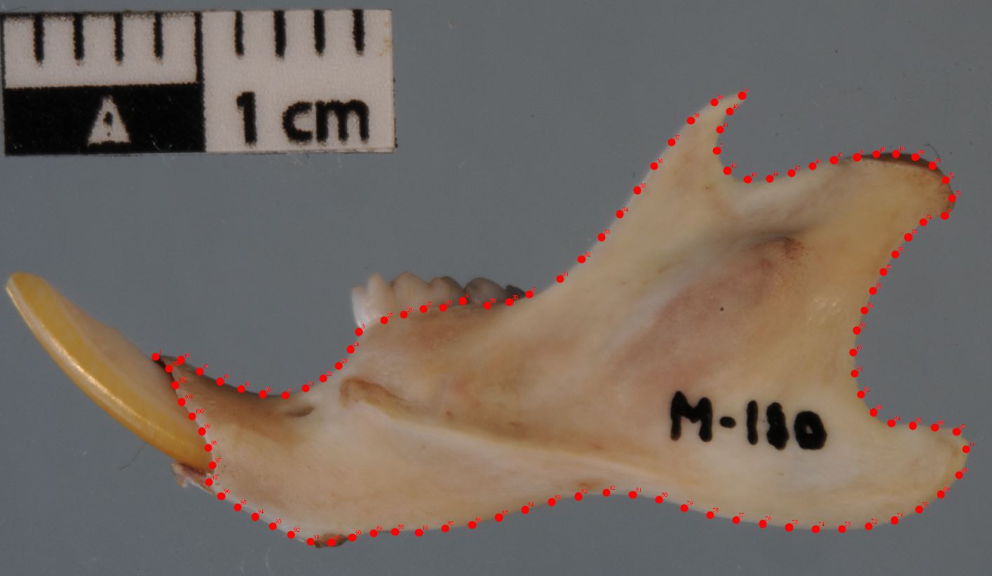
In this course, we will use the data contained in the file rats.TPS. In this file are stored the coordinates of semilandmarks taken on rats mandibles, as shown on Figure 2.1.
Figure 2.1: Protocol for semilandmarks.
NoteExercise
(Optional) Open the file rats.TPS using a text editor, inspect it and try to understand its structure.
Load this TPS file in R.
How many individuals do we have in this file?
TipSolution
In this TPS file, the rows LM=103 suggest that we have 103 landmarks per individual. Each landmark has two coordinates \((x,y)\), so that we have an array of 103 rows and 2 columns per individual. Among those landmarks, the first 15 are fixed landmarks, and the following 88 landmarks are curve semilandmarks. Finally, the file ID indicates the identifier of each individual.
Finally, we have some metadata (sex, age, weight, …) about the individuals. These data are stored in a CSV file, which is the recommended format for loading “usual” flat data in R. This data can be loaded using the built-in read.csv2() function:
          Species                   Location  Season       Weight
 Rattus rattus:159   Dry forest         :38   Dry:67   Min.   : 31.00
                     Field              : 6   Wet:92   1st Qu.: 62.00
                     Hygrophilous forest:51            Median : 98.00
                     Mesophilic forest  :49            Mean   : 94.25
                     Swamp forest       :15            3rd Qu.:120.00
                                                       Max.   :173.00
  Body_length     Tail_length         Age                Age_class  Sex
 Min.   :112.0   Min.   :143.0   Min.   :  37.10   Adult      :88   F:92
 1st Qu.:145.0   1st Qu.:191.5   1st Qu.:  87.95   Juvenile   : 5   M:67
 Median :160.0   Median :210.0   Median : 225.60   Older adult: 4
 Mean   :161.3   Mean   :204.7   Mean   : 227.04   Sub-adult  :59
 3rd Qu.:176.5   3rd Qu.:220.0   3rd Qu.: 306.10   NAs        : 3
 Max.   :205.0   Max.   :255.0   Max.   :1015.60
You may note that the levels of the (still unordered) factor Age_class are simply sorted by alphabetical order, which is the default behavior in R. The following instructions allows for a proper re-ordering of the levels:
## Re-order the age classes:meta$Age_class <-factor( meta$Age_class,ordered =TRUE,levels =c("Juvenile", "Sub-adult", "Adult", "Older adult"))table(meta$Age_class)
   Juvenile   Sub-adult       Adult Older adult
          5          59          88           4
Finally, as a (mandatory!) good practice, we should make sure that this dataframe includes the same number of individuals as the TPS file, and that they are given in the same order.
## Check dimension of CSV file:dim(meta)
[1] 159 9
## Check consistency of ordering between TPS and CSV:all(dimnames(rats)[[3]] ==rownames(rats))
[1] TRUE
I.e., the function read.csv.folder() from the package {Morpho}. In R, we can write a function with the general syntax package::function().↩︎