## Global mean shape:
Mglob <- mshape(gpa$coords)

## Shape differences with the first individual:
plotRefToTarget(Mglob, gpa$coords[, , 1], method = "TPS")
mtext("TPS")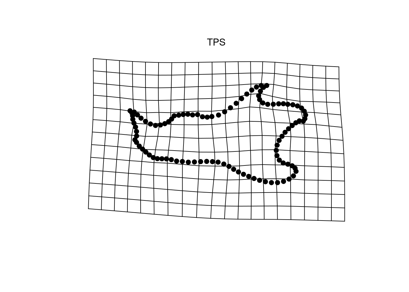
![]()
Samuel Bédécarrats 
Floriane Rémy
Frédéric Santos
Once the inter-individual variability has been described, and the factors explaining it highlighted, it can be useful to represent this morphological variation. To do so, the mean shape (also called morphotype or consensus) of each group of interest may be plotted together, so they could be compared.
Depending on the nature of the available data (2D or 3D), these morphological differences can either be represented as vectors, through a thin-plate spline or a surface color map.
The R function geomorph::plotRefToTarget() can be used to visualize the shape differences between two different landmarks configurations (as already illustrated in another section). For instance, Figure 8.1 shows the differences between the global mean shape of the sample, and one given individual.
## Global mean shape:
Mglob <- mshape(gpa$coords)
## Shape differences with the first individual:
plotRefToTarget(Mglob, gpa$coords[, , 1], method = "TPS")
mtext("TPS")The previous function can thus be used to compare the mean shapes of several groups, for instance the mean shapes of females and males.
The following code allows for the computation of female and male morphotypes respectively.
## Compute female and males morphotypes respectively.
Mfemales <- mshape(gpa$coords[ , , meta$Sex == "F"])
Mmales <- mshape(gpa$coords[ , , meta$Sex == "M"])Hint for the R code:
plotRefToTarget(Mfemales, Mmales, method = "TPS")
mtext("TPS")