## Create a dataframe-like object for subsequent analyses with geomorph:
gm.dtf <- geomorph.data.frame(
  coords = gpa$coords,
  csize = gpa$Csize,
  weight = meta$Weight,
  sex = meta$Sex,
  age = meta$Age,
  age_class = meta$Age_class,
  season = meta$Season,
  location = meta$Location
)6 Assessing the effect of covariates
In this section, we will illustrate a possible approach to assess the effect of some covariates on the shape: sex, body mass, etc. We will see in the next section a specific discussion about the effect of size on shape, also called allometry.
As a general advice, using permutation tests, or bootstrap procedures, rather than “classical” parametric tests is a good idea in morphometrics. For the rationale behind this fact, see for instance Webster and Sheets (2010).
Note that all functions for statistical inference included in {geomorph} use permutation or bootstrap tests. More generally, R packages such as {RRPP} or {vegan} implement such tests. For a very nice and friendly introduction to permutation tests and bootstrap, see for instance Zieffler, Harring, and Long (2011), Rousselet, Pernet, and Wilcox (2023) or Davison and Hinkley (1997).
Generally speaking, to assess the impact of a given covariate on shape (i.e., on Procrustes coordinates), we can for instance use:
- for a qualitative covariate (such as sex), permutation tests, PCA (as an exploratory tool), etc.;
- for a quantitative covariate (such as body mass, age in years), regression analysis, correlation tests, etc.
6.1 Reshape data
If you want to stay within the {geomorph} framework, you can use the function geomorph::gm.data.frame() to store both the (aligned) coordinates and a set of covariates in a dataframe-like object1.
If you want to be free from the {geomorph} framework and prefer handling more general and standard R objects (so that you can use them with any other R package of your choice), this code block provides an alternative:
## Create a dataframe-like object for subsequent analyses without geomorph:
gen.dtf <- data.frame(
  two.d.array(gpa$coord),
  csize = gpa$Csize,
  weight = meta$Weight,
  sex = meta$Sex,
  age_class = meta$Age_class,
  season = meta$Season,
  location = meta$Location
)
6.2 Sexual dimorphism
First, let’s begin by studying the influence of sex on shape2.
6.2.1 PCA revisited
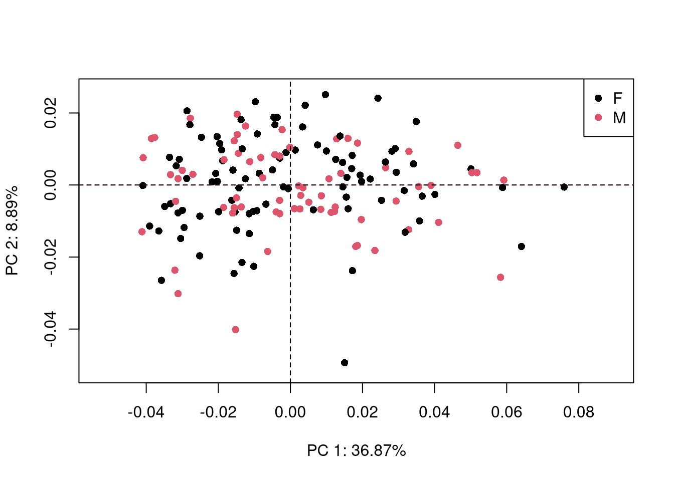
We can generate our PCA plots once again, but this time, introduce a different color for points according to the sex of the individuals. Below, the argument col allows for coloring the points according to a given factor.
## PCA with geomorph:
plot(gm.prcomp(gm.dtf$coords), pch = 16, col = gm.dtf$sex)
legend("topright", pch = 16, col = 1:2,
       legend = c("F", "M"))
{geomorph}.
How would you interpret Figure 6.1?
6.2.2 Statistical inference
To test formally the influence of sex on shape, one can use an analysis of variance of the Procrustes coordinates (or, maybe, on the coordinates of individuals on the first principal axes of the PCA, which is also a perfectly valid approach). For that, you may want to use the function geomorph::procD.lm()3:
## Analysis of variance:
procD.lm(coords ~ sex, data = gm.dtf, print.progress = FALSE) |>
  summary()
Analysis of Variance, using Residual Randomization
Permutation procedure: Randomization of null model residuals
Number of permutations: 1000
Estimation method: Ordinary Least Squares
Sums of Squares and Cross-products: Type I
Effect sizes (Z) based on F distributions

           Df       SS        MS   Rsq      F       Z Pr(>F)
sex         1 0.001649 0.0016493 0.006 0.9477 0.29544  0.383
Residuals 157 0.273228 0.0017403 0.994
Total     158 0.274877

Call: procD.lm(f1 = coords ~ sex, data = gm.dtf, print.progress = FALSE)
An alternative is the function Morpho::permudist():
permudist(pca$x, groups = gm.dtf$sex, rounds = 1000)$p.value F
M 0.55644366.3 Other qualitative covariates
6.4 Other quantitative covariates
We can also evaluate the potential effect of quantitative variables, such as age (in days), weight, etc. For the study and assessment of the relation between the shape and these quantitative covariates, regression analyses may be useful.
For instance, to study the influence of weight (in grams):
## Regression of weight on shape:
reg.weight <- procD.lm(
  coords ~ weight,
  data = gm.dtf,
  print.progress = FALSE
)
reg.weight$aov.table
Df SS MS Rsq F Z Pr(>F)
weight 1 0.061471 0.061471 0.22363 45.224 4.6768 0.001 ***
Residuals 157 0.213406 0.001359 0.77637
Total 158 0.274877
---
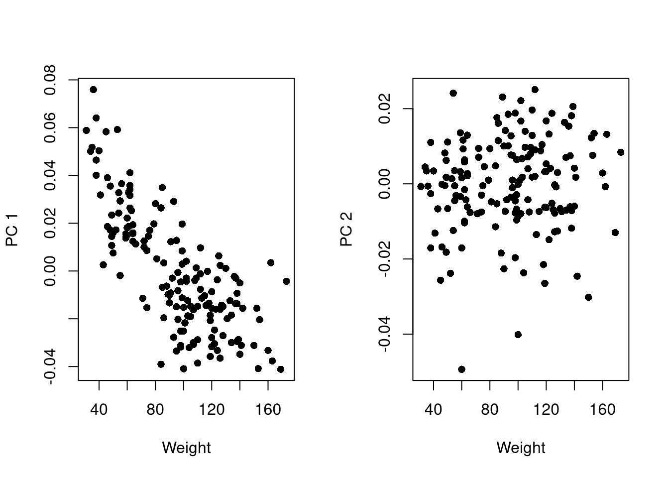
Signif. codes: 0 '***' 0.001 '**' 0.01 '*' 0.05 '.' 0.1 ' ' 1Another (simpler) approach might be to represent a scatterplot of weight and the first two axes of the PCA:
par(mfrow = c(1, 2))
plot(pca$x[, 1] ~ gen.dtf$weight, pch = 16,
     xlab = "Weight", ylab = "PC 1")
plot(pca$x[, 2] ~ gen.dtf$weight, pch = 16,
     xlab = "Weight", ylab = "PC 2")
6.5 Covariation, integration
Finally, it could be interesting in some cases to investigate the covariation between different anatomical units (e.g., mandible and skull base – this is called integration and modularity, see Klingenberg works for more information on this topic), or between an anatomical structure and quantitative covariate. In practice, these questions of covariation can often be investigated with a method called Partial Least Square analyses. See Butaric and Maddux (2016), Neaux (2017), Zlolniski et al. (2019), or Pitirri and Begun (2020) for nice examples of use of this method in biological anthropology.
Formally, this is not really a dataframe, but the data created or reshaped using this function will behave as a dataframe for all functions from the
{geomorph}package. Note that this kind of object will not make sense outside of the{geomorph}world in R.↩︎In a real study, this would probably require to control for the effect of age at the same time, or to study adults only. But one problem at a time!↩︎
Formally, this function is only a wrapper for the function
RRPP::lm.rrpp(), that we shall use later on.↩︎


