## PC1 vs. centroid size:
plot(pca$x[, 1] ~ gpa$Csize,
     pch = 16, xlab = "Centroid size",
     ylab = "PC1")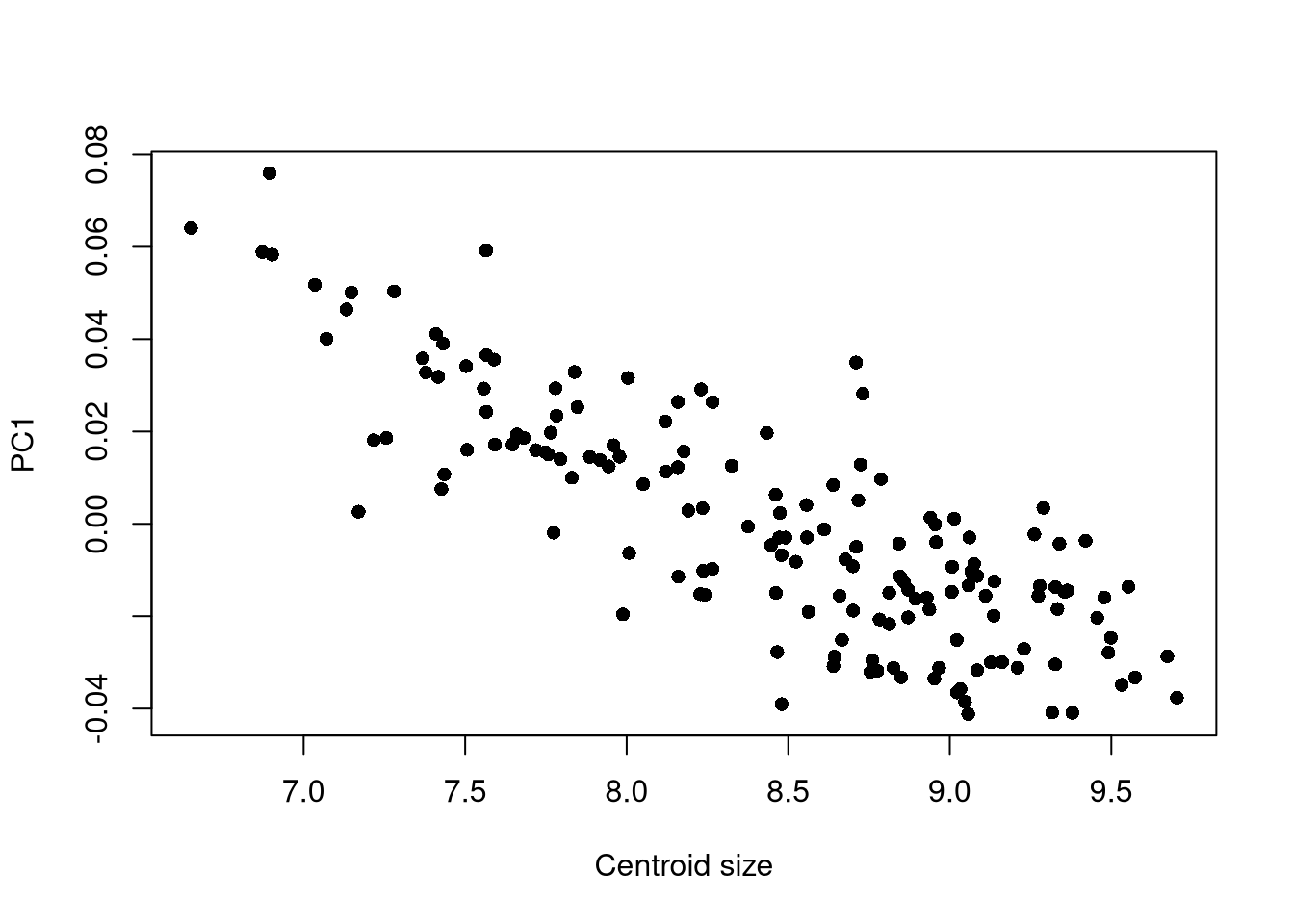
![]()
Samuel Bédécarrats 
Floriane Rémy
Frédéric Santos
Allometry is the study of size and its consequences (Gould 1966). There are three types of allometry:
It is thus a point of particular interest in studies on development or evolution.
There are several mathematical definitions of allometry and several ways of approaching it in geometric morphometry: studying the covariance of features, describing the covariance of size and shape, separating the study of size from that of shape, or considering that the effect of allometry is negligible in the study. For an overview of this topic, see for instance Klingenberg (2016).
Whatever the scientific question, allometry should be assessed and studied carefully. If the study of shape is of more relevance to the research being carried out, it is possible to “correct” for the effect of allometry, as we will see.
Among many other instances in biological anthropology, Fischer and Mitteroecker (2017) is an example of study of allometry on the human pelvis.
It is well known that the morphology os coxae strongly differs between females and males, as a response to different adaptative constraints, in particular gestation and parturition (Betti 2014; Stewart 1979; Ubelaker 1999). However, there also exists a difference in stature between females and males: within a given population, males are generally taller than females. Therefore, an interesting question could be the following: is pelvic sexual dimoprhism an allometric effect?
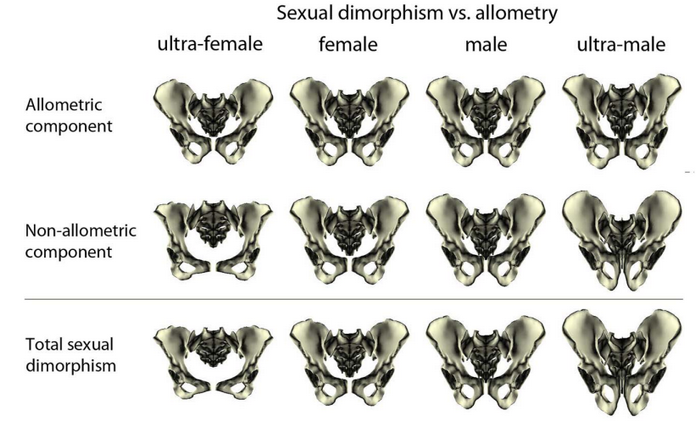
Fischer and Mitteroecker (2017) show that there is indeed an allometric effect: the pelvis becomes higher and narrower with increasing height. Since men are taller than women, part of the sexual dimorphism is explained by an allometric effect. Conversely, some traits are not related to height, such as the opening of the pelvic canal.
More technically, the allometric effect can be defined as the influence of the size (the centroid size) on the shape (the Procrustes coordinates).
Hereafter, we provide some classical ways of quantifiying allometry. Generally speaking, we should evaluate whether there is a strong and significant relationship between those size and shape. One way to do so is to use a linear model (Cornillon et al. 2023; Fox 2016), and more precisely a linear regression of shape over size. For a deeper overview of this topic, see for instance Klingenberg (2016) or Klingenberg (2022).
A first (elementary) approach would be to study the link between the first principal axis and the centroid size. This can be done, for instance, with:
## PC1 vs. centroid size:
plot(pca$x[, 1] ~ gpa$Csize,
pch = 16, xlab = "Centroid size",
ylab = "PC1")A similar approach can be performed on PC2 and subsequent axes.
However, it is also possible to inspect the whole effect of allometry by assessing the relationship between centroid size and the procrustes coordinates as a whole.
## Perform the regression analysis of Shape ~ Size:
fit <- procD.lm(
  coords ~ csize,
  data = gm.dtf,
  iter = 999
)
## ANOVA table:
fit$aov.table
Df SS MS Rsq F Z Pr(>F)
csize 1 0.07020 0.070200 0.25539 53.848 4.8678 0.001 ***
Residuals 157 0.20468 0.001304 0.74461
Total 158 0.27488
---
Signif. codes: 0 '***' 0.001 '**' 0.01 '*' 0.05 '.' 0.1 ' ' 1To conclude on the potential effect of the size on the shape, you should pay attention to the value of the Pr(>F) (a p-value, informing on statistical significance) and Rsq (i.e., \(R^2\), informing on the strength of the relationship).
Figure 7.3 shows how to represent graphically this relationship, using the method of regression scores (Drake and Klingenberg 2007). Note that each point represents an individual, and that you can color points according to a categorical variable with the col argument.
plotAllometry(fit, size = gpa$Csize,
              method = "RegScore", pch = 19)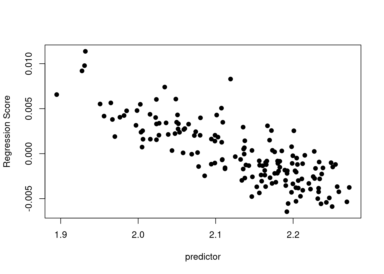
Depending on the significance and strength of the allometric effect, you can decide to run the subsequent analyses either on the raw Procrustes coordinates (to keep this potential effect of size on shape), or the residuals computed from the regression of the size over the shape (to get rid of this allometric effect and only analyze form variations). These residuals can be computed with:
## Regression residuals:
resid <- fit$residuals
As per the documentation of MorphoJ by Chris Klingenberg:
Regression is often used to correct for the effects of size on shape. If the allometric relationship between size and shape can be represented with sufficient accuracy by a linear regression of shape on size, the residuals from that regression are shape values from which the effects of size have been removed.
Therefore, analyzing the values of these residuals consists in working on size-corrected shapes.
Exercise. What can you say about the two PCAs presented in Figure 7.4 and Figure 7.5?
## PCA of shape variation (performed on raw Procrustes coordinates):
pca.shape <- PCA(gen.dtf[, 1:206], scale.unit = FALSE, graph = FALSE)
fviz_pca_ind(pca.shape, axes = c(1, 2), col.ind = gm.dtf$age_class,
             addEllipses = TRUE, label = "none", legend.title = "Age class")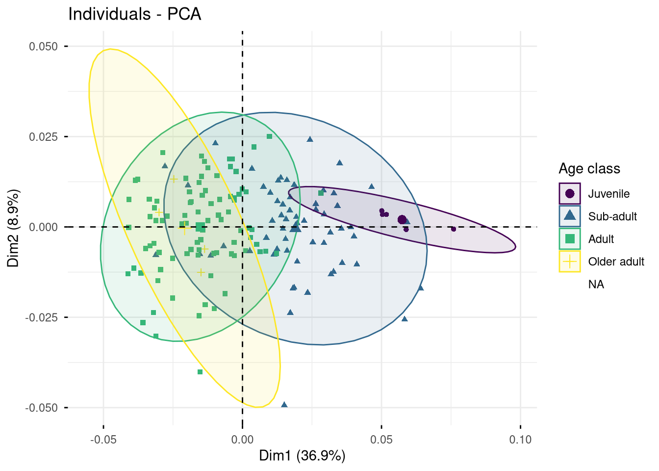
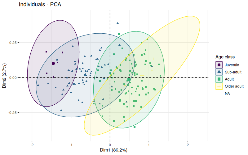
## PCA of size-corrected shape variation (performed on residuals from the regression of size over shape):
pca.sc <- PCA(resid, scale.unit = FALSE, graph = FALSE)
fviz_pca_ind(pca.sc, axes = c(1, 2), col.ind = gm.dtf$age_class,
             addEllipses = TRUE, label = "none", legend.title = "Age class")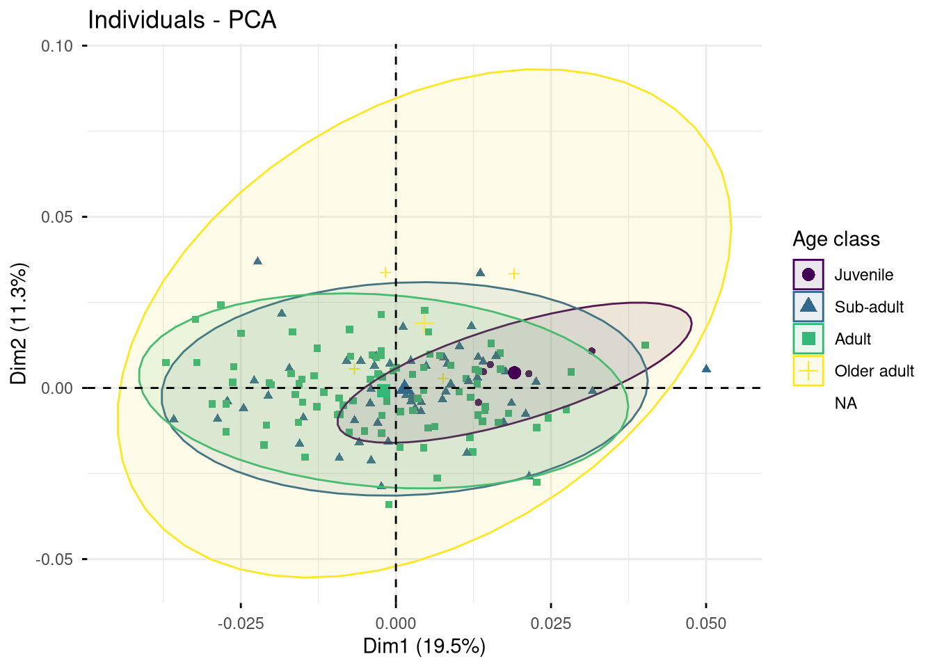
To go further in the interpretation, we can associate to these PCAs additional analyses to assess whether the selected covariate significantly contributes to the observed inter-individual variation.
Can we significantly distinguish each age class based on the mandible shape?
permudist(pca.shape$ind$coord,
          groups = gen.dtf$age_class,
          rounds = 999)$p.value
Juvenile Sub-adult Adult
Sub-adult 0.036
Adult 0.001 0.001
Older adult 0.001 0.003 0.154Can we significantly distinguish each age class based on the mandible size-corrected shape?
permudist(pca.sc$ind$coord,
          groups = gen.dtf$age_class,
          rounds = 999)$p.value
Juvenile Sub-adult Adult
Sub-adult 0.405
Adult 0.140 0.548
Older adult 0.247 0.065 0.032Finally, it could be interesting to evaluate the correlation between this covariate and the shape:
cor.test(gm.dtf$csize, gm.dtf$age, method = "pearson")
    Pearson's product-moment correlation

data:  gm.dtf$csize and gm.dtf$age
t = 13.281, df = 157, p-value < 2.2e-16
alternative hypothesis: true correlation is not equal to 0
95 percent confidence interval:
 0.6447083 0.7932121
sample estimates:
      cor
0.7273664
We could also investigate whether the centroid size significantly varies depending on the value of the covariate:
## Distribution of centroid size among age classes:
boxplot(csize ~ age_class, data = gen.dtf,
        xlab = "Age class", ylab = "Centroid size",
        main = "Distribution of the centroid size among age classes")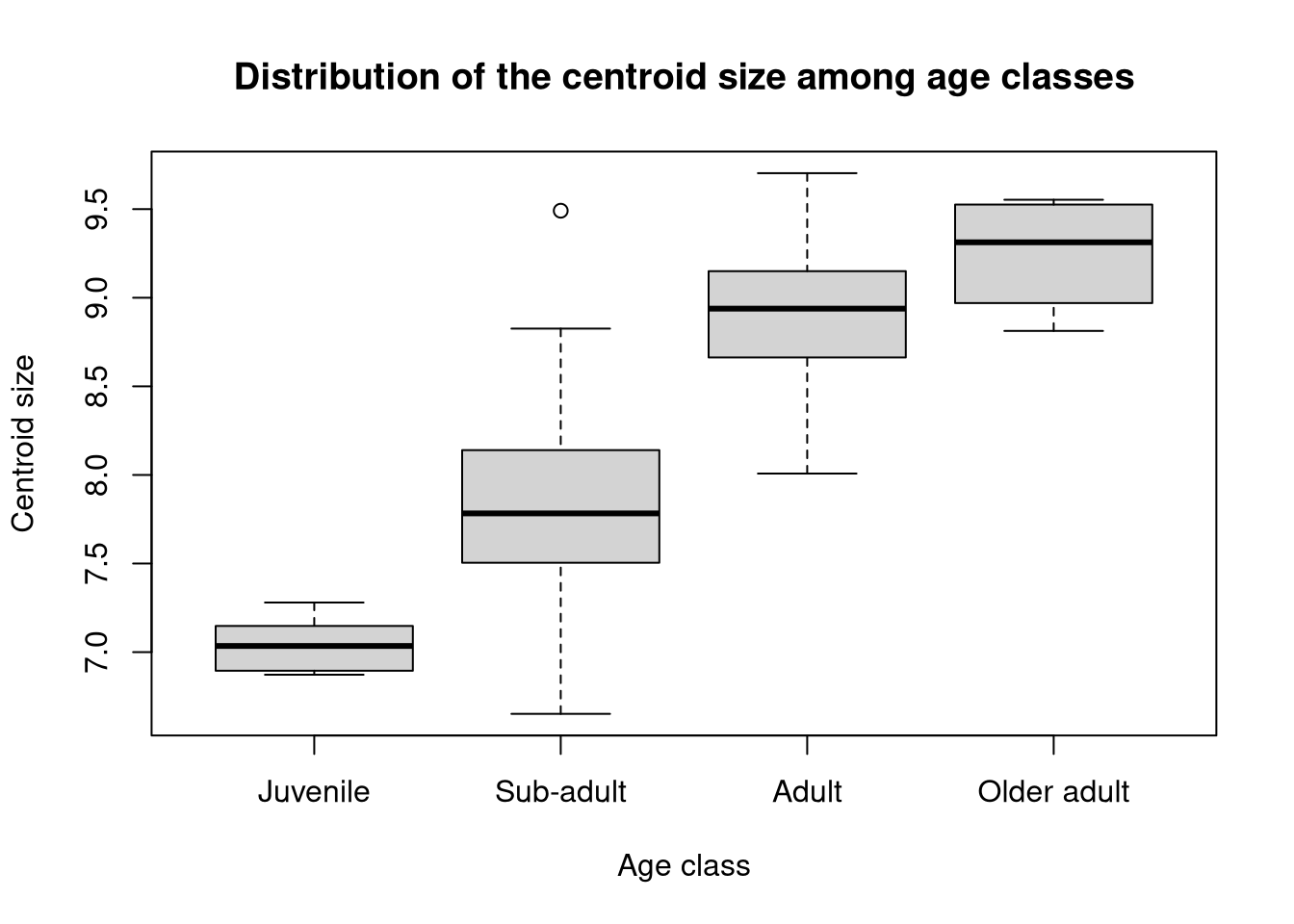
We can then test whether this distribution significantly differs between each age class1:
## ANOVA (with randomized permutations):
age.size <- lm.rrpp(csize ~ age_class, data = na.omit(gen.dtf))
anova(age.size)
Analysis of Variance, using Residual Randomization
Permutation procedure: Randomization of null model residuals
Number of permutations: 1000
Estimation method: Ordinary Least Squares
Sums of Squares and Cross-products: Type I
Effect sizes (Z) based on F distributions

           Df     SS     MS     Rsq      F      Z Pr(>F)
age_class   3 54.374 18.125 0.67526 105.35 11.655  0.001 ***
Residuals 152 26.149  0.172 0.32474
Total     155 80.523
---
Signif. codes:  0 '***' 0.001 '**' 0.01 '*' 0.05 '.' 0.1 ' ' 1

Call: lm.rrpp(f1 = csize ~ age_class, data = na.omit(gen.dtf))
Since a significant effect does show up, we may want to perform post-hoc (or pairwise) tests, to identify which pairs of age classes differ significantly.
## Pairwise comparisons:
pw.age.size <- pairwise(age.size, groups = na.omit(gen.dtf)$age_class)
summary(pw.age.size)
Pairwise comparisons

Groups: Juvenile Sub-adult Adult Older adult

RRPP: 1000 permutations

LS means:
Vectors hidden (use show.vectors = TRUE to view)

Pairwise distances between means, plus statistics
                              d UCL (95%)         Z Pr > d
Juvenile:Sub-adult    0.7792960 0.6435238 1.9427871  0.018
Juvenile:Adult        1.8680152 0.6281543 4.1874735  0.001
Juvenile:Older adult  2.2017588 0.8945375 3.5249089  0.001
Sub-adult:Adult       1.0887193 0.2369915 5.3142343  0.001
Sub-adult:Older adult 1.4224628 0.6949962 3.1184015  0.001
Adult:Older adult 0.3337435 0.6849893 0.4125271 0.356Figure 7.7 represents a PCA plot after a partial procrustes analysis: all specimens were aligned (ie centered and rotated) but there were no scaling, so that the differences in scale are preserved (R code not shown). How would you interpret this PCA, and how would you compare it to Figure 7.5 and Figure 7.4?
In practice, you might want to check the quality of this model, for instance by executing the command plot(age.size) here. But an in-depth discussion about linear models is beyond the scope of this course.↩︎