3 Procrustes superimposition

Authors

Affiliation

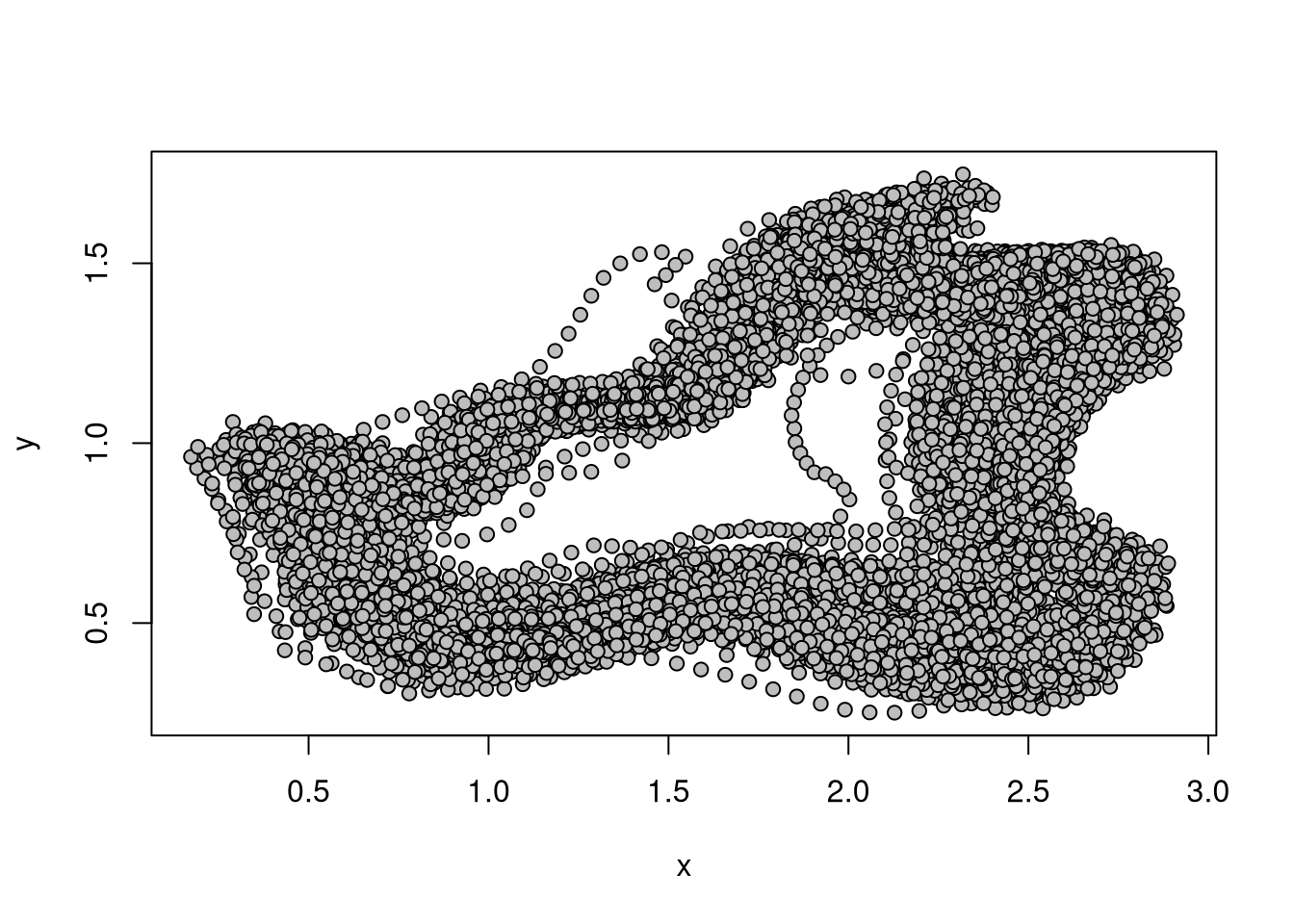
Samuel Bédécarrats

Chloé Lauer

CNRS, Univ. Bordeaux, MCC – UMR 5199 PACEA

Floriane Rémy

Frédéric Santos

CNRS, Univ. Bordeaux, MCC – UMR 5199 PACEA

Generally speaking, geometric morphometric studies are often based on the analysis of Procrustes coordinates, generated from the superimposition of the individuals, after a translation, rotation and scaling (Rohlf 1999; Ross 2004).

3.1 Procrustes analysis with R

In R, you have several options to perform a procrustes analysis on a landmarks configuration:

the function geomorph::gpagen();
the function Morpho::procSym();
the function shapes::procGPA();
and probably many others.

In all cases, your landmark data must be stored in an array.

You can perform either a complete Procrustes analysis (in this case, all individuals are scaled at the same unit centroid size), or a partial Procrustes analysis (in this case, size differences are not removed), depending on the aim of your study.

Figure 3.1 presents the landmarks of all specimens before the Procrustes superimposition.

geomorph::plotAllSpecimens(rats, mean = FALSE)

Figure 3.1: Plot of all landmark configurations, in the original coordinate system.

Note that this step should not be skipped in practice. Indeed, before beginning the analyses, it is best to make sure that there are no trivial errors in the data: did we make any mistake in the ordering of our landmarks (impairing the condition of landmarks homology)? Is there any landmark with a huge variation among specimens? Is an obvious problem with some given specimen? Figure 3.1 allows for simple checks to avoid common errors.

Just before performing the GPA, let’s make a quick recap about the 15 fixed anatomical landmarks, and the 88 curve semi-landmarks. Observe their relative position on Figure 3.2.

Figure 3.2: Fixed landmarks, and curve semi-landmarks on the mandibles.

Exercise

Perform a (complete) procrustes analysis on the R object rats previously created. If needed, you can read the help pages of the corresponding R functions; for instance with help(gpagen) and help(define.sliders) (pay extra attention to the examples presented at the end of their documentation pages).

Be careful when specifying the semi-landmarks to be slided: there are several curves that should be slided separately. Ten independent semi-landmark curves must be defined, each delimited by two anatomical landmarks. See Figure 3.2 for the indices of the (semi)landmarks associated to each curve.

Solution

## Perform a GPA with geomorph:
gpa <- geomorph::gpagen(
  A = rats,
  curves = rbind(
    define.sliders(c(1, 16:20, 2)),
    define.sliders(c(2, 21:24, 3)),
    define.sliders(c(3, 25:28, 4)),
    define.sliders(c(4, 29:30, 5)),
    define.sliders(c(5, 31:39, 6)),
    define.sliders(c(6, 40:41, 7)),
    define.sliders(c(7, 42:47, 8)),
    define.sliders(c(8, 48:53, 9)),
    define.sliders(c(9, 54:60, 10)),
    define.sliders(c(10, 61:67, 11)),
    define.sliders(c(11, 68:81, 12)),
    define.sliders(c(12, 82:87, 13)),
    define.sliders(c(13, 88:91, 14)),
    define.sliders(c(14, 92:96, 15)),
    define.sliders(c(15, 97:103, 1))
  ),
  ProcD = FALSE # you can also try TRUE to use Proc. Distance
)

An alterntive using {Morpho} instead of {geomorph} would be:

gpa2 <- procSym(
  rats,
  SMvector = c(16:103),
  outlines= c(1, 16:20, 2, 2, 21:24, 3, 3, 25:28, 4, 4, 29:30, 5,
              5, 31:39, 6, 6, 40:41, 7, 7, 42:47, 8, 8, 48:53, 9,
              9, 54:60, 10, 10, 61:67, 11, 11, 68:81, 12,
              12, 82:87, 13, 13, 88:91, 14, 14, 92:96, 15, 15, 97:103, 1)
)

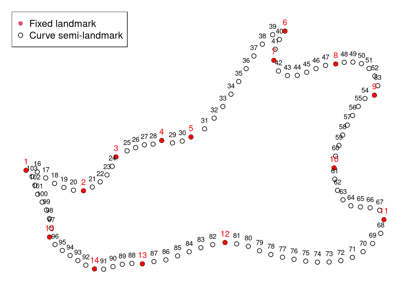
Note that if you are using semilandmarks, you can make them slide taking in consideration the bending energy with gpagen().

For curve sliding semilandmarks: the argument curves may be defined using define.sliders() to specify the indices of the semilandmarks to be slided;
For surface sliding semilandmarks: the argument surfaces should specify the indices of the semilandmarks to be slided.

3.2 Visualize the results

You can get of a summary of the results of the superimposition with:

summary(gpa)


Call:
geomorph::gpagen(A = rats, curves = rbind(define.sliders(c(1,  
    16:20, 2)), define.sliders(c(2, 21:24, 3)), define.sliders(c(3,  
    25:28, 4)), define.sliders(c(4, 29:30, 5)), define.sliders(c(5,  
    31:39, 6)), define.sliders(c(6, 40:41, 7)), define.sliders(c(7,  
    42:47, 8)), define.sliders(c(8, 48:53, 9)), define.sliders(c(9,  
    54:60, 10)), define.sliders(c(10, 61:67, 11)), define.sliders(c(11,  
    68:81, 12)), define.sliders(c(12, 82:87, 13)), define.sliders(c(13,  
    88:91, 14)), define.sliders(c(14, 92:96, 15)), define.sliders(c(15,  
    97:103, 1)))) 



Generalized Procrustes Analysis
with Partial Procrustes Superimposition

15 fixed landmarks
88 semilandmarks (sliders)
2-dimensional landmarks
11 GPA iterations to converge
Minimized Bending Energy used


Consensus (mean) Configuration

                X             Y
1   -0.1450128059  0.0347838784
2   -0.1060557881  0.0117594608
3   -0.0735868393  0.0294748167
4   -0.0401980683  0.0288498568
5   -0.0185939249  0.0261074043
6    0.0702674579  0.0711214550
7    0.0569357889  0.0496176169
8    0.1017020041  0.0465126946
9    0.1204132240  0.0196067719
10   0.0832398171 -0.0192612982
11   0.1088243962 -0.0535025736
12  -0.0153922772 -0.0398198121
13  -0.0666592033 -0.0416102160
14  -0.1010510694 -0.0380791968
15  -0.1329200528 -0.0120879758
16  -0.1386967105  0.0339715603
17  -0.1334053303  0.0303551977
18  -0.1282425761  0.0248235795
19  -0.1215798276  0.0193770001
20  -0.1140527378  0.0147115130
21  -0.0974158811  0.0119020589
22  -0.0895824761  0.0145442642
23  -0.0830294938  0.0191830342
24  -0.0782188031  0.0246296906
25  -0.0672126792  0.0302428376
26  -0.0606892088  0.0303975894
27  -0.0538557618  0.0301806341
28  -0.0469820798  0.0294926996
29  -0.0326104639  0.0275091483
30  -0.0252496873  0.0265562741
31  -0.0095992923  0.0275724913
32  -0.0009630984  0.0314220317
33   0.0074247537  0.0368182858
34   0.0157617324  0.0430505177
35   0.0242100132  0.0496652311
36   0.0329493315  0.0563355458
37   0.0421878671  0.0627213747
38   0.0521318505  0.0681988367
39   0.0623234854  0.0715344320
40   0.0684829502  0.0680896486
41   0.0605839248  0.0601790839
42   0.0591898677  0.0455079631
43   0.0661033750  0.0427260820
44   0.0747357628  0.0419815615
45   0.0833921353  0.0427161045
46   0.0908438240  0.0445398059
47   0.0967474272  0.0462159446
48   0.1082347507  0.0472859569
49   0.1156708444  0.0464770274
50   0.1223395008  0.0426404725
51   0.1259540752  0.0356526893
52   0.1265392879  0.0274025592
53   0.1241362366  0.0213729471
54   0.1159099909  0.0181671545
55   0.1105049668  0.0157950963
56   0.1046277149  0.0120920366
57   0.0988470222  0.0071899309
58   0.0934788857  0.0014827915
59   0.0888934314 -0.0049171880
60   0.0854144979 -0.0118430831
61   0.0826921790 -0.0265089633
62   0.0840134610 -0.0335291873
63   0.0876400159 -0.0394351976
64   0.0935700849 -0.0430278194
65   0.0998842527 -0.0451686811
66   0.1053353981 -0.0472672552
67   0.1084441319 -0.0499980551
68   0.1054437593 -0.0597802299
69   0.0998667407 -0.0651544190
70   0.0923478915 -0.0690891643
71   0.0836977680 -0.0710930716
72   0.0744583813 -0.0711300953
73   0.0648971533 -0.0698196536
74   0.0552894351 -0.0676405968
75   0.0457851135 -0.0648625396
76   0.0365081053 -0.0615399251
77   0.0274635736 -0.0578226312
78   0.0186799644 -0.0537240136
79   0.0101028151 -0.0495483260
80   0.0016044545 -0.0455998456
81  -0.0069192233 -0.0422747132
82  -0.0225811001 -0.0390381295
83  -0.0297979598 -0.0389237392
84  -0.0372528471 -0.0392994832
85  -0.0448047795 -0.0399228587
86  -0.0523225368 -0.0406100522
87  -0.0596220532 -0.0412727487
88  -0.0737892170 -0.0403269137
89  -0.0807112800 -0.0388287303
90  -0.0874670050 -0.0380188675
91  -0.0943283911 -0.0380858213
92  -0.1078572386 -0.0345842322
93  -0.1143729684 -0.0299743445
94  -0.1206536743 -0.0249419155
95  -0.1267369083 -0.0200921582
96  -0.1321910396 -0.0157969191
97  -0.1319722836 -0.0066263871
98  -0.1336519373  0.0003904277
99  -0.1362805239  0.0076885120
100 -0.1390843533  0.0144088119
101 -0.1407614185  0.0210714498
102 -0.1416074634  0.0270703259
103 -0.1428265612  0.0317716418

Note that, in particular, this gives you the consensus (or mean shape) of all individuals.

For a more graphical output, you can use:

plot(gpa)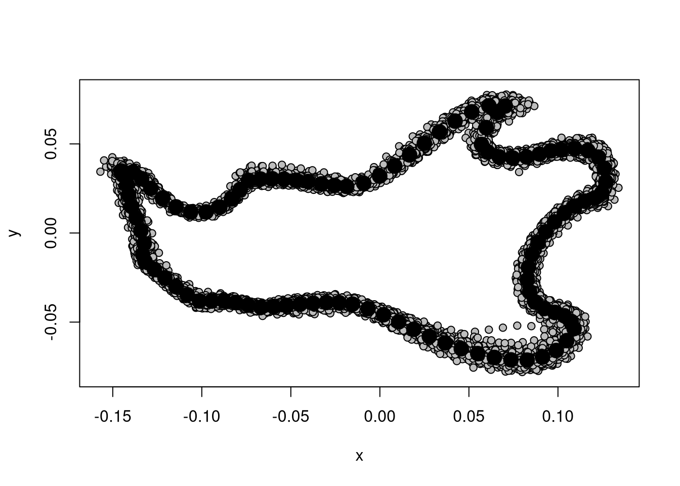

Figure 3.3: Mean shape and landmark configurations after procrustes superimposition.

You can compare this result to Figure 3.1.

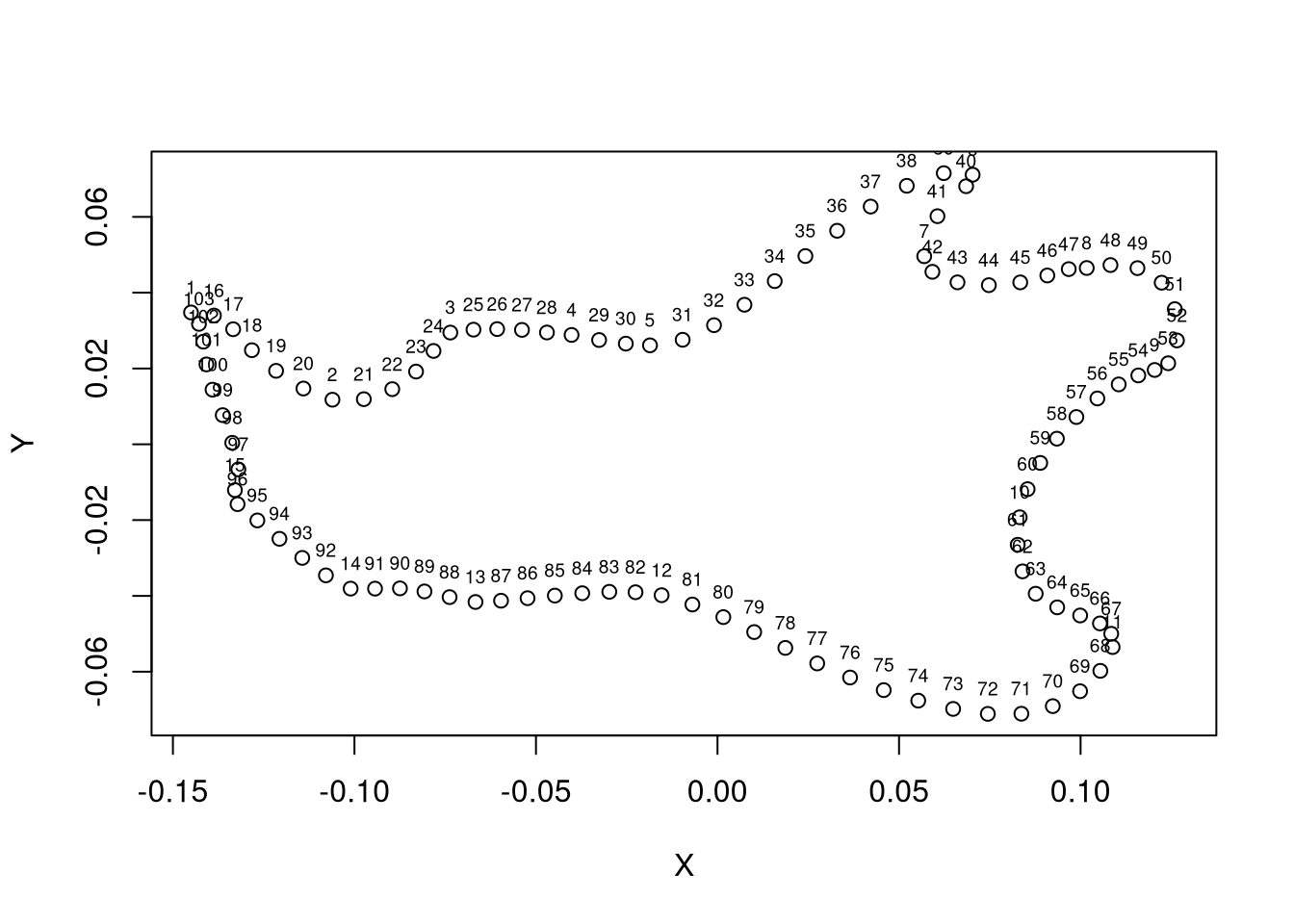
Finally, Figure 3.4 shows clearer view of the mean shape, which is useful to check whether fixed landmarks have not been wrongly slided:

plot(gpa$consensus)
text(gpa$consensus, labels = 1:103, cex = 0.6, pos = 3)

Figure 3.4: A simpler visualization of the mean shape after procrustes superimposition.